Joint Error Rate calibration
Simulations for one and two-sample tests
P. Neuvial
2018-03-27
Source:vignettes/jointErrorRateCalibration_simulations.Rmd
jointErrorRateCalibration_simulations.RmdThis vignettes illustrates the following points
- simulation of one- and two-sample Gaussian equi-correlated observations
- computation of test statistics by randomization
- calibration of Joint-Family-Wise Error Rate (JER) thresholds
We start with two-sample tests because we believe they are used more frequently.
library("sanssouci")
#set.seed(0xBEEF) # for reproducibility
library("ggplot2")
Parameters:
m <- 5e2
n <- 30
pi0 <- 0.8
rho <- 0.3
SNR <- 3
We use the function SansSouciSim to generate Gaussian
equi-correlated samples. We then ‘fit’ the resulting SansSouci
object
Two-sample tests
Simulation
obj <- SansSouciSim(m, rho, n, pi0, SNR = SNR, prob = 0.5)
obj
## 'SansSouci' object:
## Number of hypotheses: 500
## Number of observations: 30
## 2 samples
##
## Truth:
## 100 false null hypotheses (signals) out of 500 (pi0=0.8)We perform JER calibration using the linear (Simes) template , where for
where is the cdf of the distribution. Note that is the one-sided -value associated to the test statistics .
Calibration
B <- 1000
alpha <- 0.2
cal <- fit(obj, alpha = alpha, B = B, family = "Simes")
cal
## 'SansSouci' object:
## Number of hypotheses: 500
## Number of observations: 30
## 2 samples
##
## Truth:
## 100 false null hypotheses (signals) out of 500 (pi0=0.8)
## Parameters:
## Test function: rowWelchTests
## Number of permutations: B=1000
## Significance level: alpha=0.2
## Reference family: Simes
## (of size: K=500)
##
## Output:
## Calibration parameter: lambda=0.2051593The output of the calibration is the following SansSouci
object. In particular:
-
cal$inputcontains the input simulated data (and the associated truth) -
cal$paramcontains the calibration parameters -
cal$outputcontains the output of the calibration, including-
p.values: test statistics calculated by permutation -
thr: A JER-controlling family of (here ) elements -
lambda: the -calibration parameter
-
Because we are under positive equi-correlation, we expect for the Simes family.
cal$output$lambda## 20%
## 0.2051593
cal$output$lambda > alpha## 20%
## TRUEPost hoc confidence bounds
The fitted SansSouci object contains post hoc confidence
bounds:
##   x label stat bound
## 1 1 Simes   TP     1
## 2 2 Simes   TP     2
## 3 3 Simes   TP     3
## 4 4 Simes   TP     4
## 5 5 Simes   TP     5
## 6 6 Simes   TP     6
We compare it to the true number of false positives among the most significant items, and to the Simes bound without calibration
cal0 <- fit(obj, alpha = alpha, B = 0, family = "Simes")
oracle <- fit(obj, alpha = alpha, family = "Oracle")

confs <- list(Simes = predict(cal0, all = TRUE),
              "Simes+calibration" = predict(cal, all = TRUE),
              "Oracle" = predict(oracle, all = TRUE))
plotConfCurve(confs, xmax = 200, legend.title = "Template")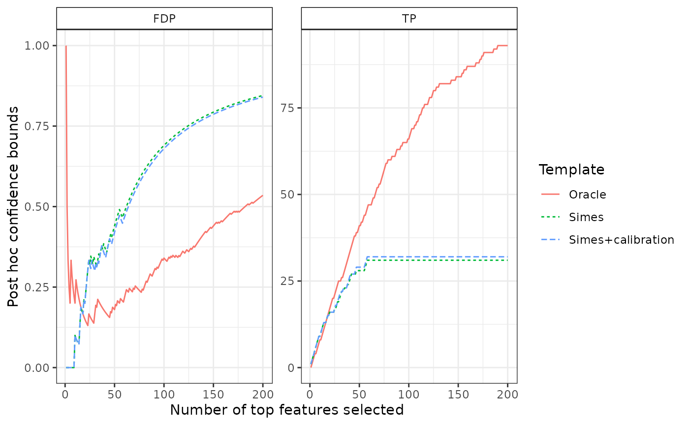
One sample tests
The code is identical, except for the line to generate the
observations (where we do not specify a probability of belonging to one
of the two populations using the prob argument); moreover
it is not necessary to specify a vector of categories ‘categ’ in
‘calibrateJER’.
obj <- SansSouciSim(m, rho, n, pi0, SNR = SNR)
obj
## 'SansSouci' object:
## Number of hypotheses: 500
## Number of observations: 30
## 1 sample
##
## Truth:
## 100 false null hypotheses (signals) out of 500 (pi0=0.8)
cal <- fit(obj, alpha = alpha, B = B, family = "Simes")
cal
## 'SansSouci' object:
## Number of hypotheses: 500
## Number of observations: 30
## 1 sample
##
## Truth:
## 100 false null hypotheses (signals) out of 500 (pi0=0.8)
## Parameters:
## Test function: rowZTests
## Number of permutations: B=1000
## Significance level: alpha=0.2
## Reference family: Simes
## (of size: K=500)
##
## Output:
## Calibration parameter: lambda=0.382704Again we expect .
Confidence curves
The associated confidence curves are displayed below:
cal0 <- fit(obj, alpha = alpha, B = 0, family = "Simes")
oracle <- fit(obj, alpha = alpha, family = "Oracle")

confs <- list(Simes = predict(cal0, all = TRUE),
              "Simes+calibration" = predict(cal, all = TRUE),
              "Oracle" = predict(oracle, all = TRUE))
plotConfCurve(confs, legend.title = "Template")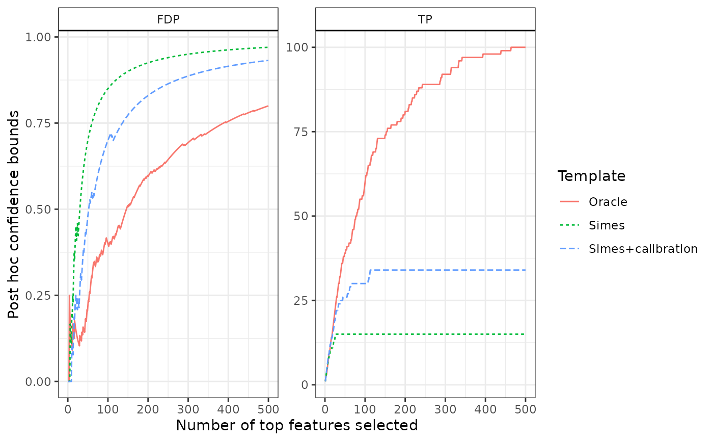
Session information
## R version 4.5.1 (2025-06-13)
## Platform: x86_64-pc-linux-gnu
## Running under: Ubuntu 24.04.2 LTS
##
## Matrix products: default
## BLAS:   /usr/lib/x86_64-linux-gnu/openblas-pthread/libblas.so.3
## LAPACK: /usr/lib/x86_64-linux-gnu/openblas-pthread/libopenblasp-r0.3.26.so;  LAPACK version 3.12.0
##
## locale:
##  [1] LC_CTYPE=C.UTF-8       LC_NUMERIC=C           LC_TIME=C.UTF-8
##  [4] LC_COLLATE=C.UTF-8     LC_MONETARY=C.UTF-8    LC_MESSAGES=C.UTF-8
##  [7] LC_PAPER=C.UTF-8       LC_NAME=C              LC_ADDRESS=C
## [10] LC_TELEPHONE=C         LC_MEASUREMENT=C.UTF-8 LC_IDENTIFICATION=C
##
## time zone: UTC
## tzcode source: system (glibc)
##
## attached base packages:
## [1] stats     graphics  grDevices utils     datasets  methods   base
##
## other attached packages:
## [1] ggplot2_3.5.2    sanssouci_0.16.0
##
## loaded via a namespace (and not attached):
##  [1] vctrs_0.6.5        cli_3.6.5          knitr_1.50         rlang_1.1.6
##  [5] xfun_0.52          generics_0.1.4     textshaping_1.0.1  jsonlite_2.0.0
##  [9] labeling_0.4.3     glue_1.8.0         htmltools_0.5.8.1  ragg_1.4.0
## [13] sass_0.4.10        scales_1.4.0       rmarkdown_2.29     grid_4.5.1
## [17] tibble_3.3.0       evaluate_1.0.4     jquerylib_0.1.4    fastmap_1.2.0
## [21] matrixTests_0.2.3  yaml_2.3.10        lifecycle_1.0.4    compiler_4.5.1
## [25] RColorBrewer_1.1-3 fs_1.6.6           pkgconfig_2.0.3    farver_2.1.2
## [29] systemfonts_1.2.3  lattice_0.22-7     digest_0.6.37      R6_2.6.1
## [33] pillar_1.11.0      magrittr_2.0.3     bslib_0.9.0        Matrix_1.7-3
## [37] withr_3.0.2        gtable_0.3.6       tools_4.5.1        matrixStats_1.5.0
## [41] pkgdown_2.1.3      cachem_1.1.0       desc_1.4.3